Based on: Gregori, J., Dynamic Arterial Spin Labeling Measurements of Physiological Parameters Permeability and Oxygenation, Dissertation, University of Heidelberg, 2009
1.1 Arterial Spin Labeling
Arterial Spin Labeling (ASL) is a non-invasive imaging technique capable of measuring perfusion. This is a great advantage over contrast agent based methods. The basic principle of ASL is to employ the blood water itself as contrast agent to measure perfusion. The longitudinal magnetization of the blood water is prepared proximally of the perfused regions, i.e. usually it is inverted by a 180° pulse. Subsequently, the prepared blood flows to the readout region and the delivered magnetization can be acquired after an inflow time TI by common readout modules. (TI is equivalent to the inversion time in the last chapters, but has the additional meaning of inflow in ASL.) ASL usually involves the acquisition of a label image (with preparation of inflowing blood water spins) and a control image (without preparation), the difference of which is the perfusion weighted output image.
1.1.1 Two basic techniques: Continuous and Pulsed Arterial Spin Labeling
The concept of Arterial Spin Labeling was first proposed by [Williams et al. – 1992]. In this original approach, blood water is labeled by using a flow-driven adiabatic inversion. This labeling technique will flip the magnetization of water molecules with a certain velocity, while stationary tissue is saturated. (For a detailed description, cf. [Bernstein et al. – 2004].) The rf pulse length is typically greater than one second. The labeling efficiency is reduced by geometrical imperfections of the rf pulse and pulsatile velocity differences of the blood flow and ranges from 80-95%. Since there is always “fresh” labeled blood delivered, the readout region will tend to reach a steady state. This technique is known as Continuous ASL (CASL).
An alternative is Pulsed ASL (PASL), where the magnetization is prepared in a large region by applying a short inversion pulse [Edelman et al. – 1994]. The labeling efficiency is generally higher then in CASL. However, while the blood is flowing into the readout region, the prepared magnetization decays with T1. This leads to smaller signal when longer inflow times are chosen.
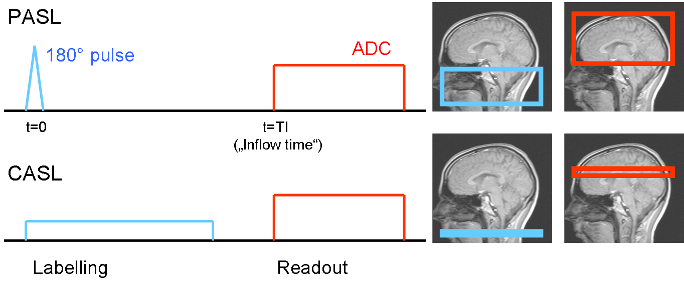 Fig. 1: Sketch of the two basic ASL techniques; in PASL, a larger region is labeled for a short time; the readout module can in both cases be chosen arbitrarily 2- or 3-dimensional
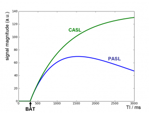
Fig. 2: Theoretical ASL signal from one voxel depending on the inflow time TI; labeled blood arrives in the voxel at TI=BAT (bolus arrival time); at later TI, the PASL curve shows T1 decay while CASL reaches a steady state.
1.1.2 Blood flow and perfusion: the General Kinetic Model
Blood flow is measured in units of ml/min and denotes the amount of blood per time flowing through a vessel. Perfusion is the amount of blood delivered to a certain amount of tissue, commonly measured in ml/100g/min.
The delivery of blood in Arterial Spin Labeling experiments can be described by the General Kinetic Model [Buxton et al. – 1998]. A good review is given by [Petersen et al. – 2006]. It includes the delivery function c(t), the residue function r(t), which describes the washout of labeled blood from the voxel, and a term m(t), which describes the decay of magnetization. The observed signal in a voxel is the convolution of the delivery function with the tissue response r(t)*m(t):

The integral can be solved analytically if simple assumptions are made. In the most common approach for pulsed Arterial Spin Labeling, the delivery function starts when the blood bolus arrives in the voxel, at BAT (“bolus arrival time”), and ends after the bolus length BL, at BAT+BL = τd. BAT highly depends on the brain region. Outflow is modeled as an exponential decay assuming a certain probability of the water molecule of leaving the voxel at time t. m(t) simply represents the longitudinal relaxation in the voxel. The describing functions are modeled as:

where α is the inversion ratio (the proportion of spins actually flipped by the 180° pulse), CBF the perfusion (usually measured in ml/100g/min), λ the tissue partition constant (the amount of tissue per volume, for grey matter approx. 0.9, cf. e.g. [Tofts – 2003]), and R1_bl, R1_ex relaxation constants in arterial blood and extra-vascular space (i.e. tissue), respectively.
Solving Equation (1) yields

The theoretical inflow curve for t<τd is shown in Fig. 2.
This is, however, only a basic model describing blood delivery to a voxel by uniform flow from one source. It describes the inflow of the blood through the vasculature, but assumes an immediate transfer of the water molecules from blood to tissue space, as soon as a water molecule arrives in the voxel (“fast exchange”). The choice of function m(t) in Equ. (2) does not include multi-compartment or transfer effects. The solution can therefore be considered a single compartment model. However, such effects can be included in m(t) before solving the convolution.
1.1.3 Magnetization Transfer: STAR and FAIR
Magnetization transfer (MT) is an effect which, in ASL, can lead to magnetization of stationary brain tissue in the readout slab. Water protons bound to macromolecules have a much broader frequency range (cf. Fig. 3) than free water protons. A labeling pulse, which is off-resonant in respect to the readout slab, can therefore still affect magnetization of the bound water molecules there. The two pools can exchange magnetization, via water diffusion or spin-spin interaction. Thereby, the magnetization of the free water protons is modified, and the free water proton magnetization will contribute to the readout signal.
The MT effect is used in MT-imaging, where it is used to estimate the bound water pool size, which hints to the presence of macromolecules. This can point to pathological changes in tissue composition.
 Fig. 3: Symbolic representation of the free (dotted line) and bound (solid line) water proton pools in brain tissue. An off-resonant rf pulse can excite bound water molecules, which can exchange their magnetization with the free water pool. Image taken from [Tofts – 2003].
In ASL, the MT effect is an important detail to be considered. The RF inversion pulse, which is off-resonant to the readout region, is only needed for the label acquisition. MT effects, which occur during labeling, but not during the control image, contribute dramatically to the perfusion weighted difference image. Therefore, methods to compensate MT effects had to be developed.
In the first PASL publication presented above, the idea was to apply the inversion pulse also in the control acquisition, but distal to the readout region. It is assumed that the MT effects are symmetric and therefore cancel out in the difference image. This is of course only practical for thin imaging slices, not for larger readout slabs. The technique is known as STAR (signal targeting with alternating radio frequency, after [Edelman et al. – 1994]).
 Fig. 4: The FAIR labeling scheme
One of the subsequently proposed MT compensation techniques is FAIR (flow alternating inversion recovery, [Kwong et al. – 1995] and [Kim – 1995]) Here, in the labeling case, a global inversion pulse is employed, thus labeling inside and outside the readout region. For the control image, a slice selective inversion pulse is used, inverting only the magnetization in the readout slab. In the difference image, this cancels out and the prepared magnetization of inflowing spins remains. FAIR is a technique which can also be used for larger readout slabs and 3D imaging. Label and control are also known as non-selective and slice selective acquisitions in FAIR.
1.1.4 Background suppression
At two time points between inversion and readout, additional global inversion pulses are applied as background suppression pulses. The timing of the pulses is optimized to null the tissue signal with a certain T1 at the time of readout TI. A schematic curve of M|| is shown in Fig. 5.

Fig. 5: Schematic magnetization curves with and without background suppression; blood signal starts at M||=-1 after inversion and decays with T1blood=1500 ms. Tissue signal starts at M||=0 after post-labeling saturation and relaxes with T1tissue=800 ms.
If one inversion pulse is employed it can be optimized to null exactly one characteristic T1. With two pulses, two different T1 tissue types can be nulled simultaneously, with correct choice of the timing, etc. However, there is no analytical solution for the inversion times of arbitrary T1 and TI. The flip angles of the inversion pulses need not be exactly 180°, but can also be optimized for maximal signal suppression [Ogg et al. – 1994].
1.1.5 Effect of varying BAT and Q2TIPS
One crucial point in planning an ASL experiment is the choice of TI. In the above considerations, acquisitions are done at exactly one fixed TI. The resulting difference from the labeled and unlabeled images is perfusion weighted. However, the signal curves depend on TI (cf. Fig. 2), and also on characteristic properties varying from voxel to voxel. Especially, BAT varies in a large range between brain regions, commonly with differences of up to one second. This leads to underestimation of perfusion in areas with larger BAT. On the other hand, choosing a long TI where all voxels are assumed to be filled with blood, will lead to substantially lower SNR. Thus, the perfusion weighted image is not directly proportional to the real perfusion map. For quantification, errors have to be taken into account and corrected. The effect is depicted in Fig. 6, where the schematic signal curves of three different voxels is shown. The blue and red curves show voxels with same perfusion value, but different BAT. The green curve shows a voxel with half the perfusion. At a chosen inflow time of TI = 2000 ms, the green signal curve is higher than the red one, despite of the significantly lower perfusion.

Fig. 6: Characteristic inflow curves of three voxels, with different arrival times and perfusion values.
Wong et al proposed to apply saturation pulses (called Q2TIPS or QUIPSS II – “Quantitative imaging of perfusion using a single subtraction, second version“) after a certain time BL (“bolus length”) to truncate the blood bolus. This circumvents fresh labeled blood from flowing into the imaging slab for times t>BL. Is BL chosen such that TI-BL>BAT for all voxels, all voxels are subject to the same temporal length of the inflow bolus and the effects of varying BAT cancel out.
The idea of the application of Q2TIPS in the above ASL scheme is slightly different. In PASL, the bolus of inverted blood is in principle arbitrarily long, spatially and temporally. In practice, however, because of imperfect slice profiles and coil geometry, blood far away from the readout center will not be perfectly inverted. The truncation of the bolus at a certain time BL is therefore a mean to prepare a known bolus shape.
Besides quantification, there is another positive effect of applying the Q2TIPS pulses directly before readout. Any signal from outside the readout slab which could disturb in the image acquisition is saturated. This is especially important because the labeling pulses are applied outside the readout region and would lead to image artifacts.
1.1.6 An optimized pulsed ASL labeling and readout scheme

Fig. 7: Schematic pulse diagram of the optimized PASL-FAIR scheme
A: The inversion pulse is slice selective in case of the control image and non-selective for the labeling image.
B: After inversion, the readout region is saturated. This prepares a homogenous uniform magnetization in the readout region and also saturates any possible MT-effects there.
C: Stationary tissue is suppressed by two background suppression 180° pulses which are optimized to null tissue signal at t = TI.
D: At t=BL (bolus length), the blood bolus is truncated by application of Q2TIPS saturation pulses. Also, signal from outside the readout slab is suppressed.
E: At t = TI, a 3D-GRASE single shot readout module acquires an image with whole-brain coverage.
In 2005, Günther et al. presented an optimized ASL preparation scheme in conjunction with a 3D-GRASE readout module [Günther et al. – 2005]. As mentioned above, care has to be taken to reduceor MT effects. Another basic issue in ASL is signal strength. The blood signal compared to tissue signal makes only a few percent. Both drawbacks are addressed in the presented approach.
Fig. 7 shows a schematic pulse diagram of the ASL sequence. This scheme is run twice, for the label- and control image. In both cases a 180° inversion pulse is applied to prepare the ASL signal. Like in the FAIR scheme, in one case the pulse is slice selective so none of the inflowing blood spins is labeled. Afterwards, post-labeling saturation pulses are applied. In the slice selective case, all previously prepared magnetization is saturated, while in the non-selective case only magnetization outside the imaging slab remains. The saturation also suppresses any MT effects in the readout region.
1.1.7 ASL time series
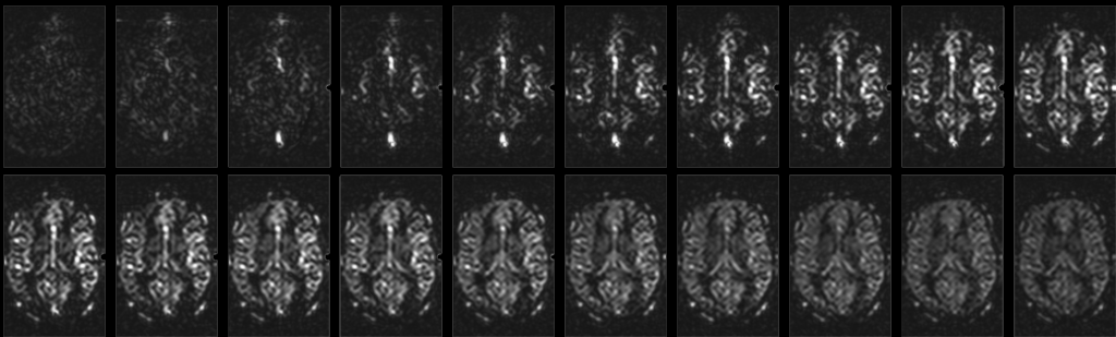
As mentioned above, varying BAT is a source of error in perfusion quantification. While there are ways to correct for these errors in a certain BAT range (like Q2TIPS), it is not sufficient in many cases. Especially cerebro-vascular diseases can lead to an uncommonly large BAT in affected areas. In these cases, it is desirable to get a detailed view on the dynamics of blood inflow. A solution to that is to acquire the perfusion weighted ASL images repeatedly with varying inflow times, thus sampling a time series of the signal evolution.

Fig. 8: ASL time series dataset; Inflow time steps range from TI=100 ms to TI=2000 ms, with a step size of 100 ms. In the first images, voxels with larger vessels appear bright. As blood is delivered to the tissue via the capillaries, on the later time steps the signal is more uniformly distributed in the tissue.
 Fig. 9: Typical data points from one voxel. The Buxton model from Equ. (1) can be fitted to the voxel data along the inflow time axis.
Typical images and data are shown in Fig. 8 and Fig. 9. The model fit yields perfusion values which also depend on the fitted bolus arrival times.
References:
Bernstein, M. A., K. F. King and J. Z. Xiaohong (2004). Handbook of MRI Pulse Sequences.
Buxton, R. B., L. R. Frank, E. C. Wong, B. Siewert, S. Warach and R. R. Edelman (1998). “A general kinetic model for quantitative perfusion imaging with arterial spin labeling.” Magn Reson Med 40(3): 383-96.
Edelman, R. R., B. Siewert, M. Adamis, J. Gaa, G. Laub and P. Wielopolski (1994). “Signal targeting with alternating radiofrequency (STAR) sequences: application to MR angiography.” Magn Reson Med 31(2): 233-8.
Günther, M., K. Oshio and D. A. Feinberg (2005). “Single-shot 3D imaging techniques improve arterial spin labeling perfusion measurements.” Magn Reson Med 54(2): 491-8.
Kim, S. G. (1995). “Quantification of relative cerebral blood flow change by flow-sensitive alternating inversion recovery (FAIR) technique: application to functional mapping.” Magn Reson Med 34(3): 293-301.
Kwong, K. K., D. A. Chesler, R. M. Weisskoff, K. M. Donahue, T. L. Davis, L. Ostergaard, T. A. Campbell and B. R. Rosen (1995). “MR perfusion studies with T1-weighted echo planar imaging.” Magn Reson Med 34(6): 878-87.
Ogg, R. J., P. B. Kingsley and J. S. Taylor (1994). “WET, a T1- and B1-insensitive water-suppression method for in vivo localized 1H NMR spectroscopy.” J Magn Reson B 104(1): 1-10.
Petersen, E. T., I. Zimine, Y. C. Ho and X. Golay (2006). “Non-invasive measurement of perfusion: a critical review of arterial spin labelling techniques.” Br J Radiol 79(944): 688-701.
Tofts, P. (2003). Quantitative MRI of the Brain.
Williams, D. S., J. A. Detre, J. S. Leigh and A. P. Koretsky (1992). “Magnetic resonance imaging of perfusion using spin inversion of arterial water.” Proc Natl Acad Sci U S A 89(1): 212-6.